WAYS OF MAPPING / INTO THE EARTH
How to map
the inside
of Earth.
The deepest maps begin with something that reaches the surface. Follow a signal into a world we cannot photograph.
NASA’s Earth ObservatorySource & rights +
Blue Marble 2002 — western hemisphere. NASA Science.
NASA imagery credited to NASA’s Earth Observatory; no third-party copyright notice on this source record. Public domain in the United States; NASA identifiers and endorsement are excluded. The cutaway is Cartologium’s separate illustration.
Open source record ↗A signal is not yet a picture.
On a street map, you can point to a building and then visit it. A map of the deep Earth asks for another kind of trust. Its colors stand for properties inferred from evidence: they are not colors seen through a window in the ground.
Even the familiar blue globe above is an assembled view. NASA’s 2002 Blue Marble combines satellite observations collected over several months. That composition describes the visible surface and clouds. Joining it to a cutaway does not turn the interior into a satellite image. The seam marks a change in how the image is known.
Earthquakes release seismic waves that instruments can record at the surface. A seismogram traces the instrument’s response through time. In the USGS example below, the labels identify an earlier P arrival and a later S arrival. P waves involve compression; S waves involve shear. The two types do not travel in the same way.
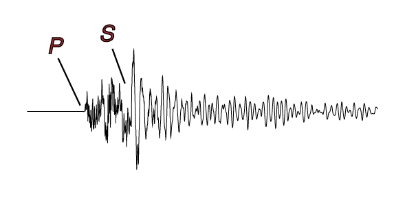
PCompression
The earlier labelled arrival
SShear
The later labelled arrival
U.S. Geological SurveySource & rights +
Example of seismic waveform. USGS Earthquake Hazards Program.
The USGS media record explicitly identifies this image as Public Domain. Its event, station, time and amplitude calibration are not identified; it is reproduced as an educational example.
Open source record ↗Look first at what this example actually provides: a trace and two labels. It does not supply a named earthquake, station, calibrated time axis or amplitude scale. Those missing particulars matter. A plausible-looking wiggle cannot, by itself, tell us where an earthquake happened or what the entire planet contains.
What was measured—and what had to be inferred?
The planet becomes a profile.
One useful simplification is to describe how properties change with depth, setting aside differences between one longitude and another. The Preliminary Reference Earth Model, or PREM, is a published global reference from 1981. Its tabulated seismic velocities make an interior readable as a profile. The figure below uses EarthScope’s version calculated for a period of one second.
DEPTH BELOW SURFACE / km
RADIAL WAVE SPEED / km s⁻¹
Outer core
2,891–5,149.5 km deep
The liquid shell of the core. The reference profile sets shear-wave speed to zero here, while compressional waves still propagate.
Model values describe an averaged Earth. The thin surface layers are difficult to resolve at this whole-planet scale.
Read the model values and method
Depth = 6,371 km − radius. The plot retains every source row, including repeated depths at boundaries. PREM includes anisotropy in the upper mantle; this figure uses its radial components only. The source’s ocean layer also has zero S-wave speed.
EarthScope model record ↗ · Original numeric table ↗| Depth (km) | P (km/s) | S (km/s) |
|---|---|---|
| 0 | 1.45 | 0 |
| 1 | 1.45 | 0 |
| 2 | 1.45 | 0 |
| 3 | 1.45 | 0 |
| 3 | 5.8 | 3.2 |
| 4 | 5.8 | 3.2 |
| 5 | 5.8 | 3.2 |
| 6 | 5.8 | 3.2 |
| 7 | 5.8 | 3.2 |
| 8 | 5.8 | 3.2 |
| 9 | 5.8 | 3.2 |
| 10 | 5.8 | 3.2 |
| 11 | 5.8 | 3.2 |
| 12 | 5.8 | 3.2 |
| 13 | 5.8 | 3.2 |
| 14 | 5.8 | 3.2 |
| 15 | 5.8 | 3.2 |
| 15 | 6.8 | 3.9 |
| 16 | 6.8 | 3.9 |
| 17 | 6.8 | 3.9 |
| 18 | 6.8 | 3.9 |
| 19 | 6.8 | 3.9 |
| 20 | 6.8 | 3.9 |
| 21 | 6.8 | 3.9 |
| 22 | 6.8 | 3.9 |
| 23 | 6.8 | 3.9 |
| 24.4 | 6.8 | 3.9 |
| 24.4 | 8.02206 | 4.39602 |
| 25 | 8.02138 | 4.39616 |
| 26 | 8.02024 | 4.39639 |
| 27 | 8.01911 | 4.39662 |
| 28 | 8.01798 | 4.39685 |
| 29 | 8.01684 | 4.39708 |
| 30 | 8.01571 | 4.39731 |
| 31 | 8.01458 | 4.39754 |
| 32 | 8.01345 | 4.39777 |
| 33 | 8.01231 | 4.398 |
| 34 | 8.01118 | 4.39823 |
| 35 | 8.01005 | 4.39846 |
| 40 | 8.00438 | 4.39962 |
| 45 | 7.99872 | 4.40077 |
| 50 | 7.99305 | 4.40192 |
| 60 | 7.98172 | 4.40422 |
| 70 | 7.97039 | 4.40653 |
| 80 | 7.95906 | 4.40883 |
| 80 | 7.95906 | 4.40883 |
| 90 | 7.94773 | 4.41113 |
| 100 | 7.93641 | 4.41344 |
| 110 | 7.92508 | 4.41574 |
| 120 | 7.91375 | 4.41805 |
| 130 | 7.90242 | 4.42035 |
| 140 | 7.89109 | 4.42265 |
| 150 | 7.87976 | 4.42496 |
| 160 | 7.86843 | 4.42726 |
| 170 | 7.8571 | 4.42957 |
| 180 | 7.84577 | 4.43187 |
| 190 | 7.83444 | 4.43417 |
| 200 | 7.82311 | 4.43648 |
| 210 | 7.81178 | 4.43878 |
| 220 | 7.80045 | 4.44109 |
| 220 | 8.55895 | 4.6439 |
| 230 | 8.57819 | 4.6509 |
| 240 | 8.59743 | 4.6579 |
| 250 | 8.61666 | 4.6649 |
| 260 | 8.6359 | 4.6719 |
| 270 | 8.65514 | 4.6789 |
| 280 | 8.67438 | 4.6859 |
| 290 | 8.69362 | 4.6929 |
| 300 | 8.71286 | 4.6999 |
| 310 | 8.7321 | 4.7069 |
| 320 | 8.75133 | 4.7139 |
| 330 | 8.77057 | 4.7209 |
| 340 | 8.78981 | 4.7279 |
| 350 | 8.80905 | 4.7349 |
| 360 | 8.82829 | 4.7419 |
| 370 | 8.84753 | 4.7489 |
| 380 | 8.86677 | 4.7559 |
| 390 | 8.886 | 4.7629 |
| 400 | 8.90524 | 4.7699 |
| 400 | 9.13392 | 4.93249 |
| 410 | 9.18511 | 4.96166 |
| 420 | 9.23631 | 4.99083 |
| 430 | 9.2875 | 5.02 |
| 440 | 9.3387 | 5.04918 |
| 450 | 9.38989 | 5.07835 |
| 460 | 9.44109 | 5.10752 |
| 470 | 9.49228 | 5.13669 |
| 480 | 9.54348 | 5.16586 |
| 490 | 9.59468 | 5.19504 |
| 500 | 9.64587 | 5.22421 |
| 510 | 9.69707 | 5.25338 |
| 520 | 9.74826 | 5.28255 |
| 530 | 9.79946 | 5.31173 |
| 540 | 9.85065 | 5.3409 |
| 550 | 9.90185 | 5.37007 |
| 560 | 9.95304 | 5.39924 |
| 570 | 10.00424 | 5.42841 |
| 580 | 10.05543 | 5.45759 |
| 590 | 10.10663 | 5.48676 |
| 600 | 10.15783 | 5.51593 |
| 600 | 10.15776 | 5.51602 |
| 610 | 10.17325 | 5.52376 |
| 620 | 10.18874 | 5.5315 |
| 630 | 10.20422 | 5.53924 |
| 640 | 10.21971 | 5.54699 |
| 650 | 10.2352 | 5.55473 |
| 660 | 10.25069 | 5.56247 |
| 670 | 10.26617 | 5.57021 |
| 670 | 10.75132 | 5.94513 |
| 685.3 | 10.79897 | 5.98986 |
| 735.3 | 10.95459 | 6.13609 |
| 771 | 11.0656 | 6.24054 |
| 771 | 11.06559 | 6.24039 |
| 785.3 | 11.09179 | 6.25067 |
| 835.3 | 11.18192 | 6.28608 |
| 885.3 | 11.26984 | 6.32065 |
| 935.3 | 11.35563 | 6.35442 |
| 985.3 | 11.43936 | 6.38742 |
| 1035.3 | 11.5211 | 6.41967 |
| 1085.3 | 11.60095 | 6.4512 |
| 1135.3 | 11.67896 | 6.48204 |
| 1185.3 | 11.75523 | 6.5122 |
| 1235.3 | 11.82983 | 6.54173 |
| 1285.3 | 11.90283 | 6.57064 |
| 1335.3 | 11.97431 | 6.59897 |
| 1385.3 | 12.04435 | 6.62674 |
| 1435.3 | 12.11304 | 6.65398 |
| 1485.3 | 12.18043 | 6.68071 |
| 1535.3 | 12.24662 | 6.70696 |
| 1585.3 | 12.31167 | 6.73276 |
| 1635.3 | 12.37567 | 6.75813 |
| 1685.3 | 12.4387 | 6.78311 |
| 1735.3 | 12.50083 | 6.80771 |
| 1785.3 | 12.56213 | 6.83197 |
| 1835.3 | 12.62269 | 6.85592 |
| 1885.3 | 12.68258 | 6.87957 |
| 1935.3 | 12.74188 | 6.90296 |
| 1985.3 | 12.80067 | 6.92611 |
| 2035.3 | 12.85902 | 6.94906 |
| 2085.3 | 12.91702 | 6.97182 |
| 2135.3 | 12.97473 | 6.99442 |
| 2185.3 | 13.03224 | 7.0169 |
| 2235.3 | 13.08963 | 7.03927 |
| 2285.3 | 13.14696 | 7.06157 |
| 2335.3 | 13.20432 | 7.08382 |
| 2385.3 | 13.26179 | 7.10605 |
| 2435.3 | 13.31944 | 7.12828 |
| 2485.3 | 13.37735 | 7.15055 |
| 2535.3 | 13.4356 | 7.17287 |
| 2585.3 | 13.49426 | 7.19529 |
| 2635.3 | 13.55341 | 7.21781 |
| 2685.3 | 13.61313 | 7.24048 |
| 2735.3 | 13.6735 | 7.26331 |
| 2741 | 13.68042 | 7.26593 |
| 2741 | 13.68044 | 7.26597 |
| 2785.3 | 13.69098 | 7.26563 |
| 2835.3 | 13.70302 | 7.2652 |
| 2885.3 | 13.71522 | 7.26471 |
| 2891 | 13.71662 | 7.26465 |
| 2891 | 8.06479 | 0 |
| 2971 | 8.19943 | 0 |
| 3071 | 8.36024 | 0 |
| 3171 | 8.51302 | 0 |
| 3271 | 8.65809 | 0 |
| 3371 | 8.79577 | 0 |
| 3471 | 8.92636 | 0 |
| 3571 | 9.05019 | 0 |
| 3671 | 9.16756 | 0 |
| 3771 | 9.2788 | 0 |
| 3871 | 9.38422 | 0 |
| 3971 | 9.48413 | 0 |
| 4071 | 9.57885 | 0 |
| 4149.5 | 9.64977 | 0 |
| 4171 | 9.66869 | 0 |
| 4271 | 9.75397 | 0 |
| 4371 | 9.835 | 0 |
| 4471 | 9.9121 | 0 |
| 4571 | 9.98558 | 0 |
| 4671 | 10.05576 | 0 |
| 4771 | 10.12295 | 0 |
| 4871 | 10.18747 | 0 |
| 4971 | 10.24963 | 0 |
| 5071 | 10.30975 | 0 |
| 5149.5 | 10.35572 | 0 |
| 5149.5 | 11.02826 | 3.50431 |
| 5153.9 | 11.02994 | 3.50549 |
| 5171 | 11.03642 | 3.51002 |
| 5271 | 11.07249 | 3.53522 |
| 5371 | 11.10541 | 3.55823 |
| 5471 | 11.1352 | 3.57905 |
| 5571 | 11.16186 | 3.59767 |
| 5671 | 11.18537 | 3.61411 |
| 5771 | 11.20576 | 3.62835 |
| 5871 | 11.223 | 3.64041 |
| 5971 | 11.23711 | 3.65027 |
| 6071 | 11.24809 | 3.65794 |
| 6171 | 11.25593 | 3.66342 |
| 6271 | 11.26063 | 3.6667 |
| 6371 | 11.2622 | 3.6678 |
Select the outer core and follow the dashed S curve. Its zero value represents a liquid region that does not transmit shear waves. The P curve continues. At the inner-core boundary, the model gives shear speed a nonzero value again. This is a property of the modeled material, not a claim that an ordinary S wave can pass straight through the intervening liquid.
The large rocky mantle is predominantly solid, even though it can deform and flow over geological time. The core has liquid and solid regions. A cutaway that colors all three in warm tones can accidentally make the planet look like a bowl of molten rock. Here the colors separate regions; they do not measure temperature.
At this scale, another choice becomes visible: the crust almost disappears. Enlarging it would make it easier to discuss, but would change the scale of the drawing. The globe emphasizes its surface rim; the numeric profile retains the source’s thin surface layers. Neither view should be mistaken for the crustal thickness beneath a particular city.
From a layered Earth to a mapped Earth.
A radial profile makes the same description available at every surface location. To investigate variation from place to place, seismic tomography combines signals that have sampled different paths. A proposed velocity model predicts travel times; comparing predictions with recordings helps researchers revise it. The result is an inferred distribution of wave speeds.
A single path leaves many possible interiors consistent with it.
Crossing paths interrogate a region from several directions.
The arrangement of the measurements matters as much as the colors in the result. Sampling geometry, noise, assumptions and the methods used to stabilize an inversion affect what can be resolved. Research on geophysical tomograms shows why a sharply drawn boundary or a fine output grid does not automatically establish equally fine knowledge.
Before reading an interior map as a landscape, find its depth, the property being plotted, the units, the reference model and the evidence for resolution. A velocity difference is not itself a photograph of a hot plume, a mineral or a reservoir of melt. Such interpretations need further physical evidence.
Read one boundary, twice.
Return to the profile and select the outer core. Compare what happens to P and S at its upper boundary. Then return to the globe. The color change and the change in the plotted properties describe the same broad boundary through different visual languages.
Return to the model ↑Mapping the inside out begins with this discipline: keep the observation, the model and the interpretation close enough to compare. It lets a reader move from a mark on a record to a structure inside the planet without losing the reasoning between them.
Sources and method.
The profile plots the published table’s depth, Vpv and Vsv columns in kilometres and kilometres per second. All rows are retained, including repeated depths at discontinuities. The broad cutaway uses a 6,371 km Earth radius, a 3,480 km core radius and a 1,221.5 km inner-core radius. It omits the model’s finer subdivisions.
The NASA composite and USGS example have individual source and rights controls. Cartologium’s cutaway, plot and sampling diagram are original visual explanations. No computed ray tracing, local tomographic model or new earthquake observation is presented.
Inspect the EarthScope model record · Read the source table. The table was retrieved on 11 October 2026. Its one-second period is a model parameter, not a record-update interval.
NASA. (2018, April 4). Blue Marble 2002 [Satellite-data composite]. https://science.nasa.gov/resource/blue-marble-2002/
Inspect the sourceWald, L. (n.d.). The science of earthquakes. U.S. Geological Survey. https://www.usgs.gov/programs/earthquake-hazards/science-earthquakes
Inspect the sourceU.S. Geological Survey. (n.d.). Inside the Earth. This dynamic Earth. https://pubs.usgs.gov/gip/dynamic/inside.html
Inspect the sourceDziewonski, A. M., & Anderson, D. L. (1981). Preliminary reference Earth model. Physics of the Earth and Planetary Interiors, 25(4), 297–356. https://doi.org/10.1016/0031-9201(81)90046-7
Inspect the sourceEarthScope Consortium. (n.d.). Seismic tomography. https://www.earthscope.org/what-is/seismology/seismic-tomography/
Inspect the sourceDay-Lewis, F. D., & Lane, J. W. (2004). Assessing the resolution-dependent utility of tomograms for geostatistics. Geophysical Research Letters, 31, L07503. https://doi.org/10.1029/2004GL019617
Inspect the sourceU.S. Geological Survey. (n.d.). Example of seismic waveform [Educational illustration]. https://www.usgs.gov/media/images/example-seismic-waveform
Inspect the image record
Editorial text and original diagrams © Cartologium. NASA and USGS imagery retain their individual source rights. Prepared 11 October 2026.